INTRODUCTION
This lab is meant to introduce a fundamental Maya concept that we admittedly gloss over in the basic curriculum: node-based representations and Maya’s Node Editor. Nodes are fundamental to getting more advanced with rigging, shading, and many other parts of the pipeline. They’re also used in a lot of 3D programs, and mastering one node-based system can help you a lot with moving to other software with similar workflows.
It can be really intimidating popping open Maya’s Node Editor and seeing tons of boxes and criss-crossing wires, but let’s break it down to make it easier to understand.
WHAT ARE NODES?
First off, let’s talk about nodes from a conceptual standpoint. Describing a 3D object is complicated, isn’t it? For anyone with more of a computer science background, you might be familiar with using collections of data structures to describe an object.
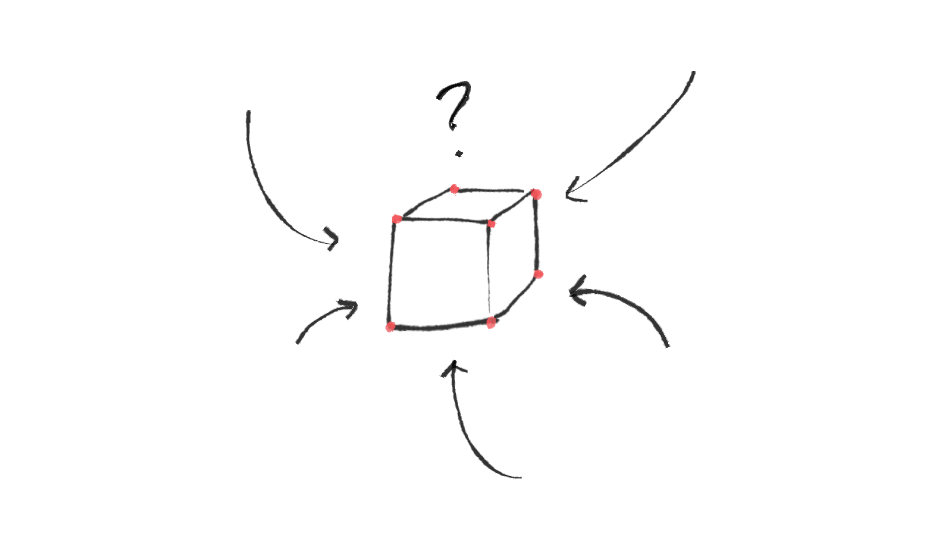
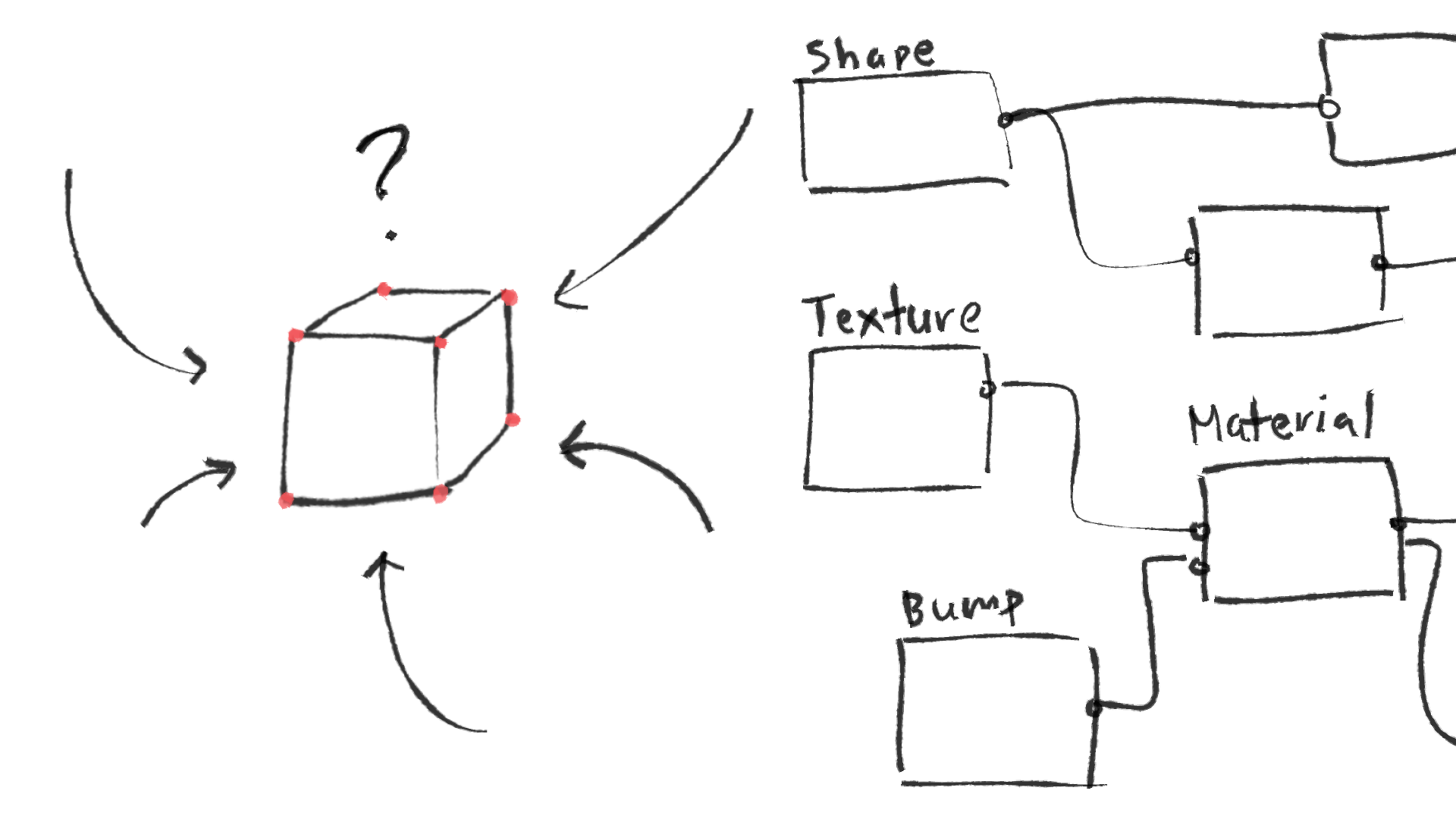
Let’s think about some properties of a 3D object. We have the positions of all the vertices, the edges connecting said vertices, and the faces which connect multiple edges. Additionally, we have the position of the object in our 3D space and other data such as rotations and scaling. We might describe its material, which, in RenderMan, is some combination of attributes such as its diffuse color, specularity, subsurface, and a host of smaller attributes.
If you’ve ever opened a .ma file in a text editor, you’ll notice all of this information typed out line by line in order to describe what’s in the file you’re looking at. Of course, editing a 3D object by editing those lines of text individually is probably not the most efficient way to work with a 3D object, and that’s where Maya comes in. Nodes are how Maya organizes all of this information about an object or scene into something that a viewer can understand.
You may actually already be familiar with some of Maya’s nodes, even if you’ve avoided looking at the Node Editor like the plague. Every time you edit an object’s vertices, edges, or faces during the modeling process with some Maya tool, you’ve been adding nodes to the object’s graph. Every time you’ve clicked on an object in the viewport then opened the Attribute Editor and flicked through the tabs, you’ve been looking at node information. Each of those tabs contain the information for a specific node related to the object.
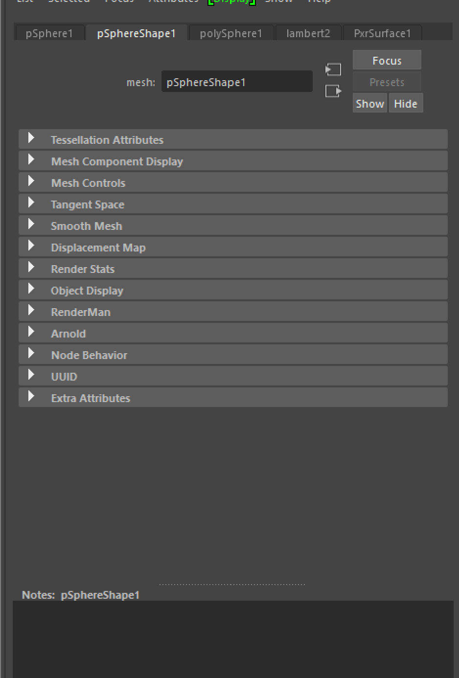
The attribute editor might give the impression that the nodes that describe an object are largely unrelated, but actually these nodes all work together and feed into one another in order to create the object you see in the viewport/render.
THE NODE EDITOR
There’s many different types of nodes, since every tool you use in Maya creates a node somewhere which serves as a record of what edits you’ve made.
Open up Maya and create a polygon sphere. You could look at its information in the attribute editor alone, but that doesn’t give you a sense of how these different attributes are related to one another. Let’s open up the Node Editor and see some more information about the object. You can find the Node Editor under Windows > Node Editor.
To view the node information about an object you currently have selected in the Viewport or Outliner, hit the “Input and output connections” button.

Which should bring up a node graph like this:
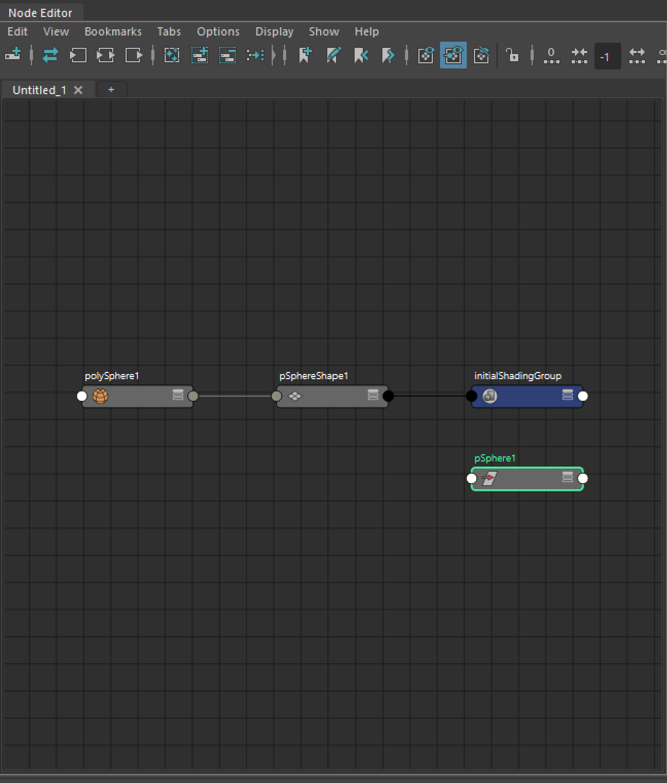
Before explaining what exactly it is we’re seeing, here’s a quick run down of some of the UI elements of the node editor. First, navigation: you can pan around with the middle mouse click and zoom in and out with your scroll wheel. Similar to the viewport, you can also click on a node and hit F to center your view of the graph on that node (or multiple nodes). Click on a node to select it, and click and drag over multiple nodes to select multiple. You can also click on the circles on the left or right of a node to create a wire, but more on that later. When a node is selected, a more detailed version of its information can be found in the attribute editor. You can also move the node around in the grid. Its position doesn’t matter, but it’s important to keep the position of nodes clean so that the wires don’t get too confusing as your graph expands.x

There’s a few different useful tools for navigating the node editor. The button labeled 1 allows you to create a new node, which will bring up a menu with a list of the available nodes in the program. The buttons labeled 2 are used to expand information about a selected node or object, either by viewing its inputs, its outputs, or both. The buttons labeled 3 let us add and remove nodes from the graph without deleting the nodes from the file. Don’t hit delete if you no longer want to view a node! That’ll remove it from the scene entirely. Hit the icon in this section instead.
The buttons labeled 4 allow us to change how much information is visible for a selected node in the node editor. You can also hit 1, 2, and 3 while selecting a node or multiple nodes to see this change, or just click on the little hamburger icon in the top right corner of any node. The buttons labeled 5 allow us to change what types of nodes will be visible in the graph by default. By default, every time you create a new node (even if it’s just using a tool outside of the node editor), it will be added to the graph. You can toggle this setting on and off with the button labeled 6.
Click on any node and expand it with the 3 key.
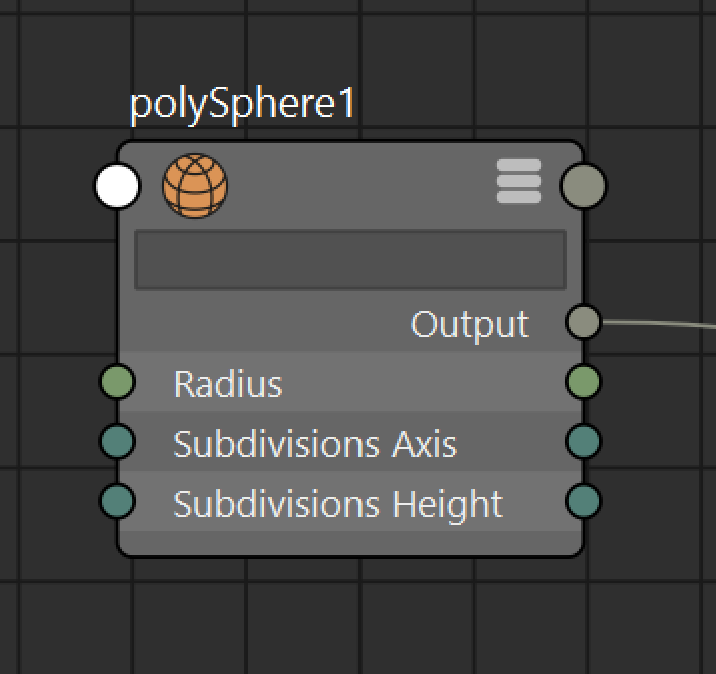
You’ll see a bunch of attributes, some of which will have circles on the left side, others with circles on the right side, and some with both. Circles on the left side of a node indicate that this attribute is an input to the node, while circles on the right side indicate that this is an output of the node. For instance, for the node I have selected above, the inputs to a polySphere object are Radius, Subdivisions Axis, and Subdivisions Height. These are also outputs, so whatever these values are set to can also get sent out from this node to a new node. Finally, we have an Output attribute, which is wired into the next node in this graph network.
NODE TYPES
Now let’s examine the node graph for our sphere. I’ve hit the 2 button while selecting all the nodes to get a bit more information.
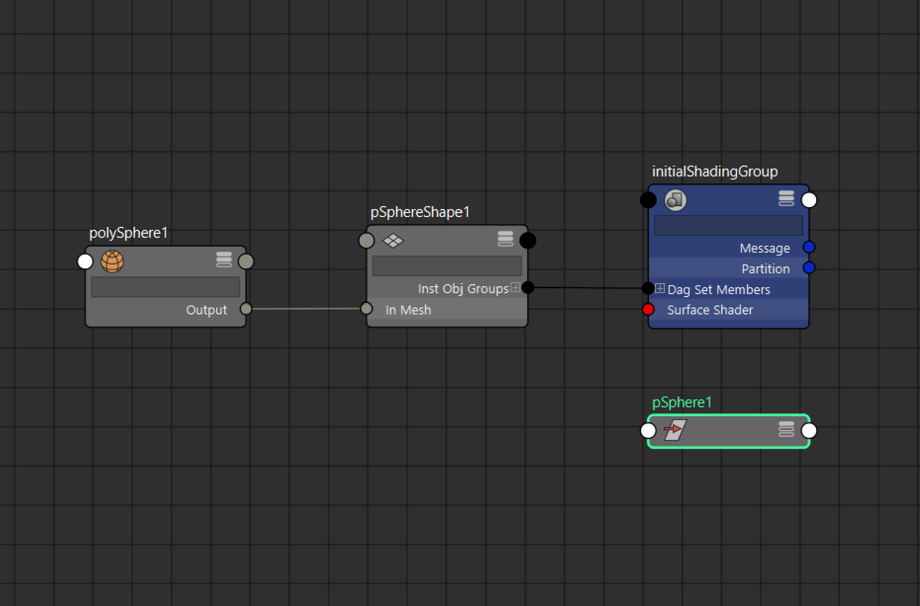
Note that whenever we select the object in the Viewport while in object mode, it highlights this node in the graph.
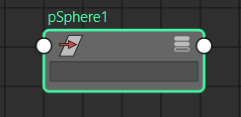
This is an object’s transform node. Whenever we interact with an object in the viewport in Object Mode, we’re working with the object’s transform node. This node stores the attributes that appear at the top of the Channel Box, such as Translate, Rotate, and Scale. The transform applies to the entire object, no matter what shape is “inside” of the transform.
Every object in Maya that appears in the viewport has a transform node and a shape node. As described in the previous paragraph, the transform node describes transformations applied to the entire object. The shape node describes the actual object, whether that’s a polygon mesh, a NURBS curve or any other type of shape object.
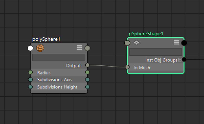
Let’s take a look at our current object’s shape node (pSphereShape1). The type is a mesh, which is indicated by the icon on the node and in the attribute editor next to the node’s name. Its input is polySphere1, which is a node that represents the sphere creation tool.
Click on the pSphere1 in the viewport and try using a tool on it, like the Smooth tool. You’ll notice that this inserts a new node into the graph, which is inserted between polySphere1 and the shape node.
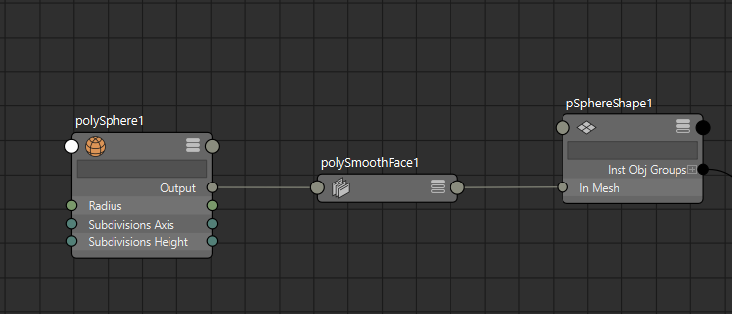
This is how Maya saves edits you make to a model, and as you continue to perform actions, this node network becomes the history of an object. You can imagine how working a complex model, like a hero character, could result in hundreds of new nodes being added. Deleting an object’s history flattens all of that information and “saves” the current vertex positions and so on into the object’s shape node.
CONNECTING NODES
Add another sphere to the viewport, and move it away from your original sphere. Select both spheres and load their networks into the Node Editor, like so.
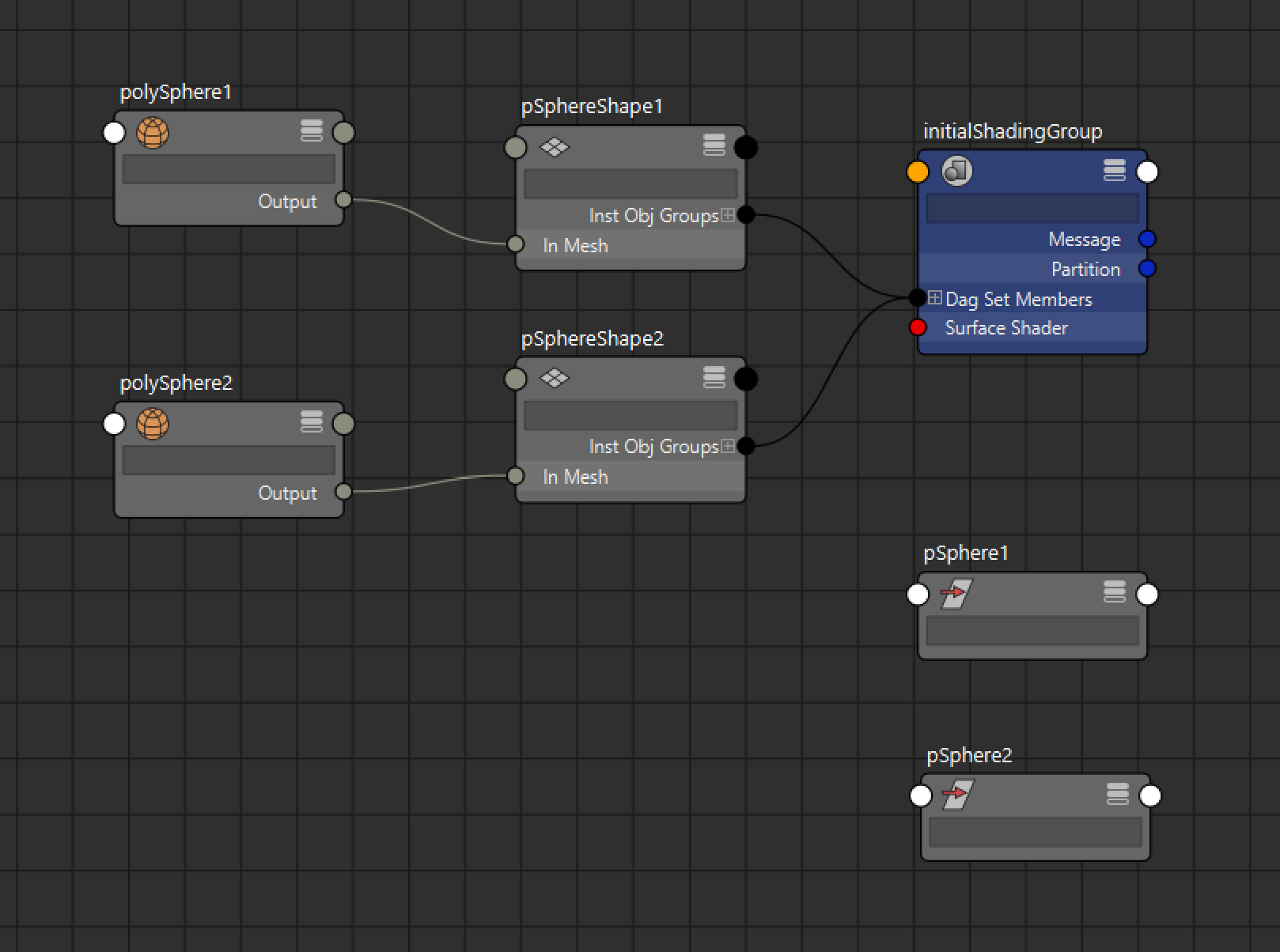
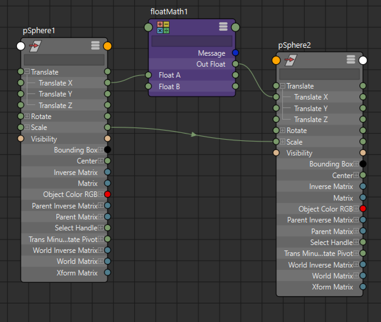
What if we wanted to make it so that Sphere2’s scale always matches Sphere1’s? We can simply move the output of Sphere1’s scale attribute into the input of Sphere2’s scale attribute by clicking on the circle on the right side of pSphere1 and connecting it to the circle on the left side of pSphere2.
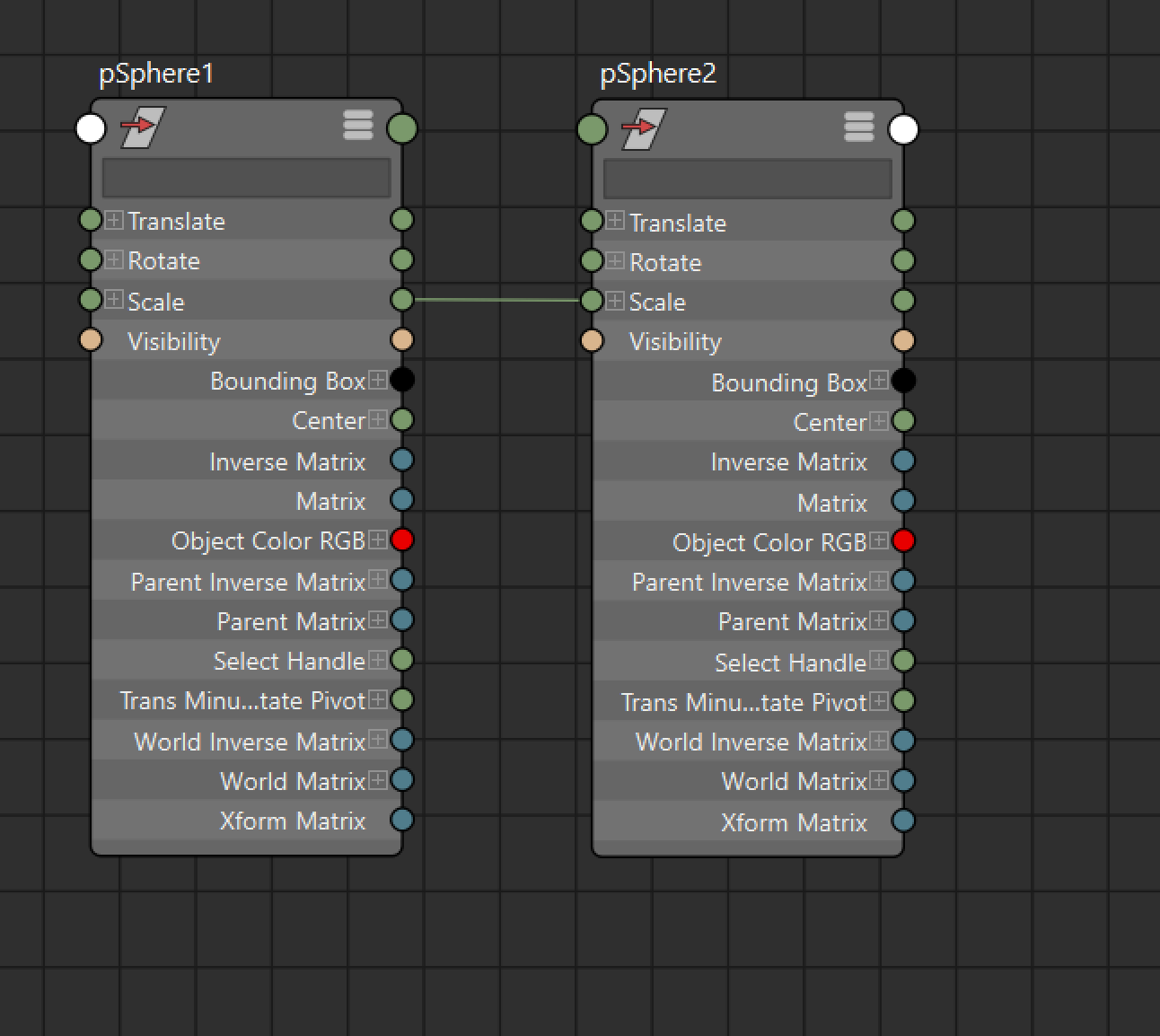
If the attribute you’re looking for doesn’t come up when switching to Full Mode (3) for a node, sometimes you’ll have to do some digging for the node attribute that you want. Hit the larger circles at the top of the node and go to “Other…” in the dropdown.
Assuming you were able to link the transform nodes like above, you should be able to scale Sphere1 in the viewport and watch Sphere2 get scaled as well.
When we wire stuff, Maya directly plugs in that attribute from the output into the input of the next node. What if we wanted to do a slightly more complex relationship, like having one object stay 3 units away from the other in a certain direction? Nodes can get a lot more powerful once we start moving beyond the regular transform and shape nodes.
Add a new node by hitting the button to bring up the node creation window. It should bring up a pane like this.
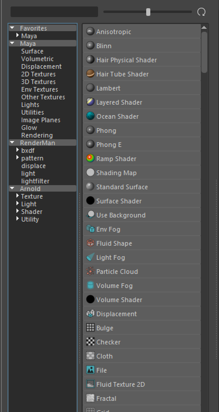
Right now, we’re looking for a node that can do some math for us, so let’s go to the Maya > Utilities part of the menu.
You may remember this from your math classes, but numbers can be stored as scalar values or vectors. In Maya, scalars are referred to as floats and vectors are referred to as colors. Since we only care about adding an offset in a single direction, and not in 3 dimensions, we can stick to doing float math.
Find a Float Math node and add it to the graph. You can also find any node you like by searching for it at the top of the Create Node pane.
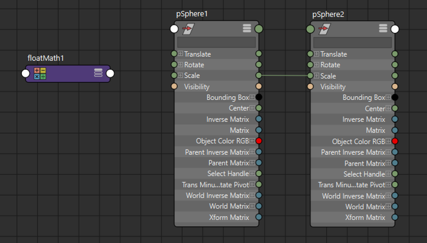
Looking at the attributes of Float Math, we can see that it takes in two float inputs and outputs another float. In the attribute editor, make sure its operation mode is set to Add. Make sure to expand your Translate attribute in both pSphere1 and pSphere2 so that you can see the X, Y, and Z components of the Translate attribute. You can do this by hitting the tiny + button to the left of the attribute. Any vector attribute in Maya can be expanded this way.
Next, let’s wire in the Translate X attribute of pSphere1 into Float A, and we can set Float B to 3, since we want one sphere to stay 3 units away from the other in the X direction. Finally, wire the output of the Float Math node into the input for pSphere2’s Translate X. That was a bunch of words and may have been difficult to process, but here’s what my graph looks like now.
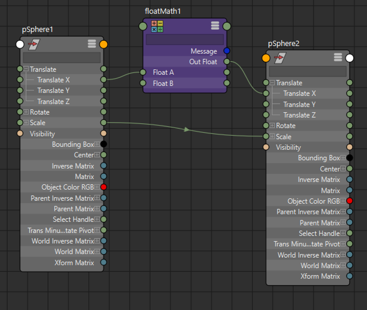
Now, you should see that pSphere2 responds to pSphere1’s translations in the X direction and copies its scale. There’s tons of different types of utility nodes in Maya, and you can use these to set up more complicated relationships between objects.
When it comes to modeling, this may not seem immediately useful, but knowing what happens behind the scene as you work is really important to understanding how 3D programs work.
Shading networks are particularly powerful, but since shader nodes are really their own world, we won’t touch on those here. The Hypershade lab will be coming up in the future for a deeper dive into those.
This guide has only scratched the surface, but hopefully from these building blocks you can begin to see how nodes unlock a lot more of Maya’s power.